


%20(1).jpg)
⚠️ IMPORTANT: This is a technical and detailed blog. If you want a more simplified and non-technical guide please refer to this article. ⚠️
Introduction
In the realm of medical imaging and machine learning, the challenge of accurately classifying Alzheimer’s disease (AD) from MRI scans stands as a crucial task. This guide aims to demystify the process, breaking down the complex steps into a more digestible format. We’ll walk through the journey of preparing MRI images for analysis and building a model that can classify these images into three categories: Alzheimer’s Disease (AD), Mild Cognitive Impairment (MCI), and Control (CN). Understanding and identifying AD early is crucial for patient care and treatment planning, making this task vital in medical research.
Index
- The Data
- Setting up our environment
- Preprocessing
- Building Classifier
- Streamlit Demo
- Conclusion
1. The Data
The MRI data can be gathered from the Alzheimer’s Desease Neuroimaging Initiative (ADNI) Database. ADNI is a longitudinal multicenter study designed to develop clinical, imaging, genetic, and biochemical biomarkers for the early detection and tracking of Alzheimer’s disease (AD) and one of its main goals is to continually administer ADNI’s innovative data-access policy, which provides all data without embargo to all scientists in the world.
The digital standard for MRI files can be found in two different formats: DICOM and NIfTI files. The difference lies in the coordinates. The DICOM image (or file) is a 2D image even though it contains a volume, but in reality, it’s a 2D image because it represents just one slice of an MRI, CT, PET, etc. The NIfTI file, on the other hand, can contain a set of these DICOM images. To provide a quick analogy, a video is a collection of frames, so when we gather all the frames, we get the video. Similarly, here we can say that DICOM images are frames, and when we put them together, we get the NIfTI file. Therefore, a NIfTI image comprehensively represents a part of the human body (in this case, the brain), containing all the slices captured using a scanner or any other method.
In this case we will use NIfTI files.
2. Setting up our Environment
Important
We will be using software that is external to python which isn’t entirely compatible with Windows. So it will be better if we use Linux or MacOS. In case you have no other choice than to use Windows, you will need to install the Windows Subsystem for Linux (WSL) which is a Windows feature that allows developers to run a Linux environment without the need for a separate virtual machine or dual booting. You will have to perform all the working within this environment rather than in windows. This means running commands in the Ubuntu terminal installed with WSL, ensuring the root folder is within WSL, if using Visual Studio Code, installing the WSL extension, etc. You can find the installation and setup guide for WSL here.
Cloning our repo
You can find a repository with all the files already prepared and a requirements.txt file in the following GitHub.
Folder tree
So, in our root folder we have three subdirectories: ADNI, atlas and preprocessing. Inside the ADNI folder we have to put all our NiFTi (MRI) files and the .csv that contains the metadata of each file (specially the class label). Inside the preprocessing, we have our 4 preprocessing python files, one for each step in our pipeline. Finally, inside the atlas folder we will put our atlas reference file for the affine registration (the explantation on this can be find on the preprocessing section).
Requirements
The requirements.txt file was separated into two files: one for the preprocessing dependencies and one for the classifier dependencies. You can install them using this files by running the following two commands in the terminal:
If you want to install only the dependencies for the preprocessing step just run the first command, if you want just the requirements for the classifier run the second command.
You can also install them manually. The dependencies are the following:
3. Preprocessing
Introduction
Before creating a model, MRI images need to be preprocessed. The main reason behind this is that MRI images have a lot of information that is not necessary for the classification model and that can even affect the classification. For example, MRI images are not images of just the brain, they also have the skull, the eyes and other tissues. In addition, MRI machines generate noise in the images, which medical professionals know they have to ignore, but machines do not, so it’s important to remove it before training a model.
Steps
- Separate NIfTI files into subdirectories according to class label
- Perform affine registration
- Skull stripping
- N4 enhanced bias correction
Step 1: Compile ADNI
The first step in our preprocessing pipeline consists in matching NIfTI files to the master metadata csv file provided by ADNI and divide each of them into sudirectories with their corresponding class label (AD, MCI, CN). For that, we first have to open our compile_adni.py file with our favorite IDE and replace at line 12 the “introduce csv file name here" with the name of the master metadata csc file.
Now we can run the python file, just by introducing in the terminal:
After running this file, a new folder will be created inside the root folder called data. Inside this folder we can find a new folder called ADNI which has 3 subdirectories (AD, CN, MCI), each of them containing the corresponding NiFTi files already segregated.
Step 3.2: Register
Our next step in the preprocessing stage is to perform the affine registration transformation. The goal of affine registration is to find the affine transformation that best maps one data set (e.g., image, set of points) onto another. In many situations data is acquired at different times, in different coordinate systems, or from different sensors. Such data can include sparse sets of points and images both in 2D and 3D, but the concepts generalize also to higher dimensions and other primitives. Registration means to bring these data sets into alignment, i.e., to find the “best” transformation that maps one set of data onto another, here using an affine transformation.
3.2.1 Installing and Setting up FSL
The first thing we have to do to perform this transformation is to install FSL. FSL is a comprehensive library of analysis tools for FMRI, MRI and diffusion brain imaging data created by the University of Oxford. You can find the installation process for MacOS, Linux and Windows (WSL) here.
After completing the installation, make sure that FSL is set up in your PATH environment variables.
3.2.2 Performing the transformation
Now that we have FSL already installed, we can perform the affine registration. For this, we will use two of the FSL tools: fslreorient2std and flirt. The first one is a simple tool designed to reorient an image to match the orientation of the standard template images (MNI152) so that they appear "the same way around" in FSLeyes. The latter is a fully automated robust and accurate tool for linear (affine) intra- and inter-modal brain image registration.
FSL doesn’t work with python, it's run through the terminal. So, for example if we wanted to run the fslreorient2std tool on one of our files we should open a terminal a right the following command:
We only use python so we don’t have to type one by one the files and run them one by one. But the only thing we are doing in python is running the commands in the terminal automatically. Moreover, we can use the multiprocess functions in python so that our CPU uses all its cores and processes multiple files at once.
To perform the transformation, we have to perform two easy tasks. The first one is to search for our reference NiFTi file for the affine registration and put it in the atlas folder. FSL comes with lots of reference images for this transformation, which our found in the following directory: FSL/data/standard. We have to select the MNI152 that goes with the type of MRI we are working with. In my case, all my MRI files were 1mm T1 MRIs, so I selected the MNI152_T1_1mm.nii file, but if for example your nifti files are 2mm T1 you should use the MNI152_T1_2mm.nii file. Once the file is inside the atlas folder, open the register.py file in the preprocessing folder and in line 66 change “name of MNI152 file” with the name of the atlas reference file you selected. In my case it should be “MNI152_T1_1mm.nii”.
Once this is done, we can now run the register.py file by introducing in the terminal:
This will create a new folder inside the data folder called ADNIReg which has 3 subdirectories (AD, CN, MCI), each of them containing the corresponding NiFTi files already transformed.
Step 3.3: Skull Stripping
MRI scans are not only of the brain, they come will lots of other information. Like the skull, the eyes, the nose, the tongue, etc., etc., etc. Although, we humans, are able to know that all that visual information has to be ignored and just focus on the brain, computers don’t have this ability so lots of unnecessary information is fed into the machine learning model which can lead to a more extensive training and a loss in the model accuracy. That’s why one of the steps in our preprocessing is performing skull stripping, which is the process of removing all this unnecessary information and just keeping the brain.
In order to perform this, we will use another tool from FSL called bet. As we said before, the FSL tools are run in the terminal so we will use python to perform it automatically in all files and speeding things up using multiprocessing.
In this step we don’t perform any special task, we just run the skull_strip.py file using the following command on the terminal:
This will use all the files in the data/ADNIReg folder, perform skull stripping on them and store them in a new folder inside the data directory called ADNIBrain. As before, inside we can find 3 subdirectories (AD, CN, MCI), each of them containing the corresponding NiFTi files.
Step 3.4: Bias Correction
N4 bias correction is a technique used to eliminate intensity inconsistencies, often referred to as “bias fields,” from medical imaging. A medical professional is capable of ignoring or identify this bias or inconsistencies, but a machine no, so they might arise from different sources like variations in scanner settings or the patient’s physical structure. Such bias fields can greatly impact the precision and dependability of image analysis. Correcting these fields enhances the overall image clarity and minimizes the impact of external variables on the analysis process.
3.4.1 Installing and Setting up ANTs
To perform this bias correction, we will use a library called Advanced Normalization Tools (ANTs), which is a very popular toolkit for processing medical images. The installation process for Linux/WSL and MacOS can be found in the following link.
3.4.2 Performing the transformation
Once ANTs is installed and the path to the bin folder is already set into the PATH environment variable, we can proceed to perform the N4 bias correction. For this, we just have to run the bias_correct.py file in the same way we ran the other files. Keep in mind that this transformation is the most expensive one computationally, so that's why you can choose to modify a little bit the python file so that it runs in batches and not all at once. For this just unncomment lines 72 to 87, comment lines 89 to 93 and change the batches variable to generate the amount of batches you want. Take into consideration that you need to know the total amount of files and subtract one. So, for example, if you want to make batches that process 200 files at a time and your total amount of files is 1615, then lines 72 to 93 should look like this:
If you want to run it all at once, just keep everything as it is.
Final result
After all the preprocessing steps are done this is the difference between the original and the processed file:
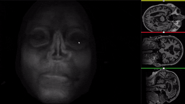
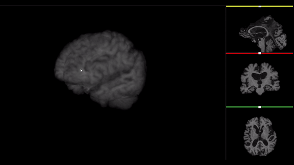
NIfTI files where open and viewed using the University of Michigan’s Brain Viewer which can be found in the following link
4. Building the Classifier
Introduction
Now that we have our preprocessing done, we can start creating our classificator. As we have seen in the preprocessing we are working with 3 different classes: Alzheimer’s Disease (AD), Mild Cognitive Impairment (MCI) and Control (CN). The issue with building an MRI classificator is that the data comes in 3D format and almost all convolutional neural networks are built to receive 2D data as input. Luckily for us we can use MONAI library to help us with this issue as it has lots of 3D convolution neural networks. In this case we will use MONAI’s DenseNet 121.
Extra requirements for using GPU
If we want to use our own GPU for training the Neural Network we will need to install some extra requirements. First of all, we will need to install CUDA, which is a parallel computing platform and programming model developed by NVIDIA for general computing on graphical processing units (GPUs). In other words, it allows us to use GPU for our training. We will be using version 11.6 which can be installed using the instructions in the following link.
We also need to install cudNN (CUDA for neural networks) which is another NVIDIA library that allows us to use CUDA for neural networks. Here you can find the explanation on how to install it.
4.1 Building the trainer
Now that we have everything ready, we can start building our Neural Network and train it! The first step is to import the necessary libraries and obtain system information:
Next we have to set the data directory. In our case all our files are located in the data/ADNIDenoise folder so we write the following:
The following step is to create a list of the paths to each file and a list of its corresponding label:
Now we can create a training, a validating and a testing data set and make the necessary transformations to it. For that, we will write the following lines:
Afterward, we need to create our DataLoaders. A DataLoader is a Pytorch data primitive that allow you to use pre-loaded datasets as well as your own data. DataLoader wraps an iterable to enable easy access to the samples. We will create a DataLoader for our training and validation sets:
Now its time to set up our DenseNet model and, in case you have a pre-trained model or you want to continue training an existing model, just uncomment the last two lines and add the path to your .pth file:
The repository comes with a pretrained model with an 86% of accuracy called 86_acc_model.pth*, which can be found in the root folder. This pretrained model can still be trained to get higher accuracy scores.*
As we said before, we are using DenseNet 121, but MONAI comes with lots of different neural networks. Here you can find all the available models. If you want to use any of them just change .DenseNet121 with the model you would like to use and adapt the hyperparameters that go with the model you choose.
Finally, we can start our training. Write the following code and adjust the parameters according to your case, like the amount of epochs:
This code will run all the epochs and store the one that has the best metric into a .pth file in the root folder called best_metric_model_classification3d_array.pth. You can run this code as many times as you want in order to keep training the model.
4.2 Testing our model
To test the accuracy of our model, we first need to create a DataLoader for the test dataset, so we run the following code:
Then we load the .pth file we want to test:
And finally, we test our model accuracy:
5. Demo
Here you can see a demo created with Streamlit and deployed in Huggingface which illustrates a little example of how this model can be used.
The demo consists of three NIFtI files: one for Alzheimer’s Desease, one for Mild Cognitive Impairment and one for Control. You can select which of the three to open and view. One the side bar you can find three slide bars which let you modify were the Coronal, the Axial and the Sagital cuts are made in MRI viewer. Then you can press the “Preprocess Image” to run all the preprocessing steps and continue playing with the slide bars using the new processed image. Finally, if you press the “Run Prediction” button the model is run and the classfication is displayed along with the probability of such prediction.
6. Conclusion
In this comprehensive guide, we navigated through the intricate process of using MRI scans for the classification of Alzheimer’s Disease, Mild Cognitive Impairment, and Control groups. We started by understanding the importance of the ADNI Database as a rich source of MRI data and the nuances of different MRI file formats like DICOM and NIfTI. This foundation set the stage for our journey into the technical realm of image processing and machine learning.
Setting up a robust environment, especially the intricacies involved with compatibility issues across different operating systems, highlighted the importance of a versatile and adaptive approach in computational research. We then delved into the preprocessing steps crucial for refining MRI data for analysis. Each step, from compiling ADNI data to affine registration, skull stripping, and bias correction, was a testament to the meticulous attention to detail required in medical imaging and data preparation.
The climax of our exploration was the construction of a classifier using DenseNet 121, a model adept at handling the complexities of 3D MRI data. We discussed the need for GPU capabilities for efficient training and the potential of different neural network architectures available in the MONAI library.
As we conclude, it’s clear that the intersection of medical imaging and machine learning holds immense potential. The methodologies and tools we discussed are just the tip of the iceberg. Future advancements may include more sophisticated neural networks, deeper integration of AI in diagnostic processes, and perhaps, a broader application of these techniques in other areas of medical imaging. As technology evolves, so will our ability to understand and combat diseases like Alzheimer’s, offering hope for earlier detection, better patient outcomes, and more informed healthcare strategies.


